
Journal
of Geographic Information and Decision Analysis, vol.1, no.1, pp. 69-82
Three
Fastest Shortest Path Algorithms on Real Road Networks: Data Structures
and Procedures
F. Benjamin Zhan
Department
of Geography and Planning, Southwest Texas State University,
San Marcos, TX 78666, USA
fz01@swt.edu
http://www.swt.edu/~fz01/
ABSTRACT It
is well known that computing shortest paths over a network is an important
task in many network and transportation related analyses. Choosing
an adequate algorithm from the numerous algorithms reported in the literature
is a critical step in many applications involving real road networks.
In a recent study, a set of three shortest path algorithms that run fastest
on real road networks has been identified. These three algorithms
are: 1) the graph growth algorithm implemented with two queues, 2) the
Dijkstra algorithm implemented with approximate buckets, and 3) the Dijkstra
algorithm implemented with double buckets. As a sequel to that study,
this paper reviews and summarizes these three algorithms, and demonstrates
the data structures and procedures related to the algorithms. This
paper should be particularly useful to researchers and practitioners in
transportation, GIS, operations research and management sciences.
KEYWORDS: shortest
path algorithms, GIS, transportation, networks
Acknowledgments This
research was supported in part by a Faculty Research Enhancement Grant
from Southwest Texas State University and in part by a copy of UNIX Arc/Info
from Environmental Systems Research Institute, Inc (ESRI). The author also
wishes to thank Boris V. Cherkassky, Andrew V. Goldberg and Tomasz Radzik
for making their one-to-all shortest paths C source codes available.
Contents
1.
Introduction
With the development of geographic information systems (GIS) technology,
network and transportation analyses within a GIS environment have become
a common practice in many application areas. A key problem in network
and transportation analyses is the computation of shortest paths between
different locations on a network. Sometimes this computation has
to be done in real time. For the sake of illustration, let us have
a look at the case of a 911 call requesting an ambulance to rush a patient
to a hospital. Today it is possible to determine the fastest route
and dispatch an ambulance with the assistance of GIS. Because a link
on a real road network in a city tends to possess different levels of congestion
during different time periods of a day, and because a patient's location
can not be expected to be known in advance, it is practically impossible
to determine the fastest route before a 911 call is received. Hence,
the fastest route can only be determined in real time. In some cases
the fastest route has to be determined in a few seconds in order to ensure
the safety of a patient. Moreover, when large real road networks
are involved in an application, the determination of shortest paths on
a large network can be computationally very intensive. Because many
applications involve real road networks and because the computation of
a fastest route (shortest path) requires an answer in real time, a natural
question to ask is: Which shortest path algorithm runs fastest on real
road networks?
Although considerable empirical
studies on the performance of shortest path algorithms have been reported
in the literature (Dijkstra 1959; Dial et al.
1979; Glover et al. 1985; Gallo and Pallottino 1988; Hung and Divoky
1988; Ahuja et al. 1990; Mondou et al. 1991; Cherkassky et
al. 1993; Goldberg and Radzik 1993), there is no clear answer as
to which algorithm, or a set of algorithms runs fastest on real road
networks. In a recent study conducted by Zhan
and Noon (1996), a set of three shortest path algorithms that run fastest
on real road networks has been identified. These three algorithms
are: 1) the graph growth algorithm implemented with two queues, 2) the
Dijkstra algorithm implemented with approximate buckets, and 3) the Dijkstra
algorithm implemented with double buckets. As a sequel to that study,
this paper reviews and summarizes these three algorithms, and demonstrates
the data structures and implementation strategies related to the algorithms.
The rest of the paper is
organized as follows. Recent evaluations, particularly the evaluation
of 15 shortest path algorithms using real road networks, are briefly reviewed
in Section 2. Network representation, the labeling method and data
structures related to shortest path algorithms in general are reviewed
in Section 3. The graph growth algorithm implemented with two queues
is described in detail in Section 4. The approximate and double bucket
implementations of the Dijkstra algorithm are reviewed in Section 5.
Concluding remarks are given in Section 6.
A network is defined as a directed graph G = (N, A) consisting of
a set N of nodes and a set A of arcs with associated numerical
values, such as the number of nodes, n=|N|, the number of arcs, m=|A|,
and the length of an arc connecting nodes i and j, denoted as l(i,j).
The shortest path problem can be stated as follows: given a network, find
the shortest distances (least costs) from a source node to all other nodes
or to a subset of nodes on the network. These shortest paths represent
a directed tree T rooted from a source node s with the characteristic
that a unique path from s to any node i on the network is
the shortest path to that node (Ahuja et al.
1993). The length of the shortest path from s to any node
i is denoted as d(i). This directed tree is called
a shortest path tree. For any network with n nodes,
one can obtain n distinctive shortest path trees. Shortest
paths from one (source) node to all other nodes on a network are normally
referred as one-to-all shortest paths. Shortest paths from
one source node to a subset of the nodes on a network can be defined as
one-to-some shortest paths. Shortest paths from every node
to every other node on a network are normally called all-to-all shortest
paths.
Although there have been a number of reported evaluations of shortest path
algorithms in the literature (e.g., Glover et
al. 1985; Gallo and Pallottino 1988; Hung and Divoky 1988), a recent
study by Cherkassky et al. (1993) is one
of the most comprehensive evaluations of shortest path algorithms to date.
They evaluated a set of 17 shortest path algorithms. In their experiment,
Cherkassky et al. coded the 17 algorithms using the C programming
language, and tested the C programs on a SUN Sparc-10 workstation.
One-to-all shortest paths can be computed by these C programs.
Readers are referred to the Cherkassky et al.
(1993) paper for more detailed descriptions about the implementation of
the algorithms. Cherkassky et al. used a number of simulated
networks with various degrees of complexity for evaluating the algorithms.
The results of their studies suggest that no single algorithm performs
consistently well on all simulated networks.
More recently, Zhan and Noon (1996) tested 15
of the 17 shortest path algorithms using real road networks. In their
evaluation, Zhan and Noon dropped two of the 17 algorithms tested by Cherkassky
et al. They did not consider the special-purpose algorithm
for acyclic networks because an arc on real road networks can be treated
bi-directional, and hence real road networks contain cycles. They
also dropped the implementation using a stack to maintain labeled
Table 1 Summary
of the 15 Algorithms Evaluated
Abbreviation
|
Implementation
|
BFM
|
Bellman-Ford-Moore
|
BFP
|
Bellman-Ford-Moore with Parent--checking
|
DKQ
|
Dijkstra's Naive Implementation
|
DKB
|
Dijkstra's Buckets -- Basic Implementation
|
DKM
|
Dijkstra's Buckets -- Overflow Bag
|
DKA
|
Dijkstra's Buckets -- Approximate
|
DKD
|
Dijkstra's Buckets -- Double
|
DKF
|
Dijkstra's Heap -- Fibonacci
|
DKH
|
Dijkstra's Heap -- k--array
|
DKR
|
Dijkstra's Heap -- R--Heap
|
PAP
|
Graph Growth -- Pape
|
TQQ
|
Graph Growth with Two Queues -- Pallottino
|
THR
|
Threshold Algorithm
|
GR1
|
Topological Ordering -- Basic
|
GR2
|
Topological Ordering -- Distance Updates
|
nodes (see the next section for descriptions about stack and labeled
nodes) because they found that this algorithm is many times slower than
the rest of the algorithms on real road networks during their preliminary
testing. These 15 algorithms are summarized in Table
1. It is not the intention of this paper to review these 15 algorithms
thoroughly. Detailed description of the algorithms can be found in
Cherkassky et al. (1993) and the references
therein.
In their evaluation, Zhan
and Noon used 21 real road networks for evaluating the shortest path algorithms.
These 21 networks included the U.S. National Highway Planning Network (NHPN)
covering the continental U.S. and 20 state-level road networks generated
from road networks in 10 states in the Midwest and Southeast of the United
States. The 10 states are Alabama (AL), Florida (FL), Georgia (GA),
Iowa (IA), Louisiana (LA), Minnesota (MN), Missouri (MO), Mississippi (MS),
Nebraska (NE), and South Carolina (SC). The 20 state-level road networks
are composed of 10 low-detail road networks and 10 high-detail road networks.
The 10 low-detail networks contain three levels of roads, including interstate
highways, principal arterials and major arterials. The 10 high-detail
networks consist of one additional level of more detailed roads in addition
to the three levels of roads contained in the low-detail networks.
The 21 networks were stored and maintained in Arc/Info GIS running on a
SUN Sparc-20 workstation under the Solaris 2.4 environment. The nodes,
arcs and arc lengths were downloaded from Arc/Info into ASCII files.
Before downloading, a check was made to ensure that the networks were fully
connected.
A summary of the 21 networks
used in Zhan and Noon's evaluation is given in Table
2. One important characteristic of a real road network is the degree
of connectivity measured by the arc-to-node ratios. It can be seen
in Table 2 that the arc-to-node ratios range from 2.66 to 3.28 in the 21
networks. The degree of connectivity in these 21 networks differ
considerably from that of simulated networks where the arc-to-node ratios
can be as high as 10 (cf., Gallo and Pallottino 1988).
In addition, there is no notable difference in the degrees of connectivity
in all 21 networks. Because the number of scans in constructing a
shortest path tree is directly related to arc-to-node ratios, it is very
important to observe this difference between the arc-to-node ratios in
real road networks and simulated networks.
The 15 algorithms were coded
in the C programming language. The C programs were based on the set of
one-to-all shortest path C programs provided by Cherkassky
et al. (1993). The set of one-to-all shortest path C codes
were modified to automatically generate all-to-all shortest paths.
The C programs were compiled with the gcc compiler version 2.5.6 using
the O4 optimization option. Zhan and Noon's experiments were conducted
on a SUN Sparc-20 workstation (model HS21 with a 125MHz Hypersparc processor
and 64 Megabytes of RAM running under the Solaris 2.4 environment).
More detailed description about the experiments can be found in Zhan
(1995) and Zhan and Noon (1996).
Based on their evaluation, Zhan and Noon suggested that the best performing
implementation for solving the one-to-all shortest path problem is Pallottino's
graph growth algorithm implemented with two queues (TQQ). They further
suggested that when the goal is to obtain a one-to-one shortest path or
one-to-some shortest paths, the Dijkstra algorithm offers some advantages
because it can be terminated as soon as the shortest path distance to the
destination node is obtained (see Section 5). Zhan and Noon recommended
two of Dijkstra implementations. The choice between the two implementations
depends on the maximum network arc lengths. They recommended the
approximate buckets implementation of the Dijkstra algorithm (DKA) for
computing one-to-some shortest paths over networks whose maximum arc length
is less than 1500. For networks whose maximum arc length is
greater than 1500, they recommended that the double buckets implementation
of the Dijkstra algorithm (DKD) should also be considered.
Table 2 Summary
of the 21 real road networks used in the evaluation
No.
|
state
|
number of nodes
|
number of arcs
|
arc/node ratio
|
maximum arc lengt
|
mean arc length
|
stnd. dev. of arc lengths
|
1
|
NE
|
523
|
1646
|
3.14
|
0.874764
|
0.215551
|
0.142461
|
2
|
AL
|
842
|
2506
|
2.98
|
0.650305
|
0.128870
|
0.114031
|
3
|
MN
|
951
|
2932
|
3.08
|
0.972436
|
0.175173
|
0.132083
|
4
|
IA
|
1003
|
2684
|
2.68
|
0.573768
|
0.119900
|
0.113719
|
5
|
MS
|
1156
|
3240
|
2.80
|
0.498810
|
0.095443
|
0.100703
|
6
|
SC
|
1784
|
5128
|
2.88
|
0.413163
|
0.062156
|
0.064389
|
7
|
FL
|
2155
|
6370
|
2.96
|
0.923088
|
0.075247
|
0.076590
|
8
|
MO
|
2391
|
7308
|
3.06
|
0.494730
|
0.090977
|
0.064761
|
9
|
LA
|
2437
|
6876
|
2.82
|
1.021526
|
0.060662
|
0.067557
|
10
|
GA
|
2878
|
8428
|
2.92
|
0.478579
|
0.068333
|
0.005668
|
11
|
LA
|
35793
|
98880
|
2.76
|
0.360678
|
0.013874
|
0.015297
|
12
|
MS
|
39986
|
120582
|
3.02
|
0.232062
|
0.015412
|
0.014000
|
13
|
NE
|
44765
|
146476
|
3.28
|
0.528283
|
0.018039
|
0.015652
|
14
|
FL
|
50109
|
133134
|
2.66
|
0.416212
|
0.011207
|
0.015264
|
15
|
SC
|
52965
|
149620
|
2.82
|
0.163557
|
0.009975
|
0.010198
|
16
|
IA
|
63407
|
208134
|
3.28
|
0.269823
|
0.015733
|
0.009220
|
17
|
MN
|
65491
|
209340
|
3.20
|
0.410925
|
0.017202
|
0.014107
|
18
|
AL
|
66082
|
185986
|
2.82
|
0.298232
|
0.011383
|
0.012410
|
19
|
MO
|
67899
|
204144
|
3.00
|
0.212470
|
0.015542
|
0.013266
|
20
|
US
|
75417
|
205998
|
2.74
|
1.500361
|
0.066084
|
0.094758
|
21
|
GA
|
92792
|
264392
|
2.84
|
0.174245
|
0.010511
|
0.000107
|
Note: The first 10 networks are low-detail
road networks (three levels of roads) from the ten states. The remaining
11 networks are the 10 high-detail road networks (four levels of roads)
from the ten states plus the US National Highway Planning Network (US).
The networks are ordered by the number of nodes (After Zhan
and Noon 1996).
The way in which an input network is represented and implemented in a shortest
path algorithm is vital to the performance of the algorithm. Past
research has proven that the forward star representation is the most efficient
data structure for representing networks (Gallo and
Pallottino 1988; Ahuja et al. 1993 p.35-36; Cherkassky et al.
1993). Two sets of arrays are used in the forward star data structure.
The first array is used to store data associated with arcs, and the second
array is used to store data related to nodes. All arcs of a network
in question are maintained in a list and are ordered in a specific sequence.
That is, arcs emanating from nodes 1, 2, 3, ..., are ordered sequentially.
Arcs emanating from the same node can be ordered arbitrarily, however.
All information associated with an arc, such as starting node, ending node,
cost, arc length and capacity are stored with the arc in some way (e.g.,
corresponding arrays or linked lists).
For the array of nodes,
a total of n+1 elements are needed. The i-th element associated
with node i, pointer(i), stores the sequential number (in
the above arc list) of the first arc emanating from node i.
There are a few exceptions: 1) for a node i that has no outgoing
arc, pointer(i) is set equal to the content of the next element
in the array, i.e., pointer(i) = pointer(i+1); and 2) for consistency,
the following convention is adopted, i.e., pointer(1)=1 and pointer(n+1)=m+1.
The labeling method is a central procedure in most shortest path algorithms
(Gallo and Pallottino 1988; Ahuja et al. 1993,
p.96). The output of the labeling method is an out-tree from
a source node, s, to a set of nodes. This out-tree is constructed
iteratively, and the shortest path from s to i is obtained
upon termination of the method. Three pieces of information are maintained
for each node i in the labeling method while constructing a shortest
path tree: the distance label, d(i), the parent node, p(i),
and the node status, S(i). The distance label, d(i),
stores the upper bound of the shortest path distance from s to i
during iteration. Upon termination of an algorithm, d(i) represents
the unique shortest path from s to i. The parent node
p(i) records the node that immediately precedes node i in
the out-tree. The node status, S(i), can be one of the following:
unreached, temporarily labeled and permanently labeled.
When a node is not scanned during the iteration, it is unreached.
Normally the distance label of an unreached node is set to positive infinite.
When it is known that the currently known shortest path of getting to node
i is also the absolute shortest path we will ever be able to attain,
the node is called permanently labeled. When further improvement
is still expected to be made on the shortest path to node i, node
i is considered only temporarily labeled. It follows
that d(i) is an upper bound on the shortest path distance to node
i if the node is temporarily labeled; and d(i) represents
the final and optimal shortest path distance to node i if the node
is permanently labeled.
At the beginning of the
iterations in the labeling method, a directed out-tree is initialized and
the initial values of the above parameters d(i), p(i) and
S(i) are set for source node s and every other node i
accordingly (Ahuja et al. 1993).
During the scanning process, when a node i is scanned, the distance
label of a successor node j is checked and an attempt is made to
lower the distance label, d(j), of node j. If
d(j) can be lowered, the out-tree is updated by changing the parent
node of j to i, that is, p(j) = i. Because d(j)
is lowered, node j should ultimately become permanently labeled.
The iteration continues until all nodes become permanently labeled.
Upon termination of the iterations, the out-tree becomes a shortest path
tree. Formally, the scanning operation for node i can be described
below.
Procedure ScanningOperation(i)
begin
for all successor nodes of i do
if d(i) + l(i,j) < d(j) then
begin
d(j) = d(i) + l(i,j);
p(j) = i;
S(j) = labeled;
end
S(i) = permanently labeled;
end
The performance of a particular shortest path algorithm partly depends
on how the basic operations in the labeling method are implemented.
Two aspects are particularly important to the performance of a shortest
path algorithm: 1) the strategies used to select the next temporarily labeled
node to be scanned, and 2) the data structures utilized to maintain the
set of labeled nodes. We briefly review these two aspects in this
subsection. Readers can refer to Gallo and
Pallottino (1988) and Ahuja et al.
(1993) for more detailed discussions on these topics.
Strategies commonly used
for selecting the next temporarily labeled node to be scanned are "First
In First Out" (FIFO), "Last In First Out" (LIFO) and "Best-First-Search"
(Gallo and Pallottino 1988). It is fairly
easy to see from the names of the first two search strategies that the
oldest node in the set of temporarily labeled nodes is selected first in
a FIFO search strategy and the newest is selected first in a LIFO strategy
at each iteration. In the best-first-search strategy, the node with the
minimum distance label from the set of temporarily labeled nodes is
considered as the best node.
A number of data structures
can be used to manipulate the set of temporarily labeled nodes in order
to support these strategies. These data structures include arrays,
singly and doubly linked lists, stacks, buckets and queues. Detailed
definitions and operations related to these data structures are standard
knowledge and are well documented in the literature (e.g., Sedgewick
1990; Ahuja et al. 1993, pp.765-787). Therefore, we only
selectively review some of them. A singly linked list contains
a collection of elements. Each element has a data field and a link
field. The data field contains information to be stored, and the
link field contains a pointer pointing to the next element in the list.
A doubly linked list differs from a singly linked list in that each element
in a doubly linked list contains two pointers. One pointer points
to the previous element in the list, and another pointer points to the
next element in the list. Stack is another special type of list which
only allows removal and addition of an element at one end of the list.
This end of the list is normally called the top of a stack. The bucket
data structure is described in detail in Section 5 because it is related
to two of the three recommended algorithms, namely, the approximate and
double bucket implementations of the Dijkstra algorithms.
A queue is a special type
of list which allows the addition of an element at the tail and the deletion
of an element at the head. A priority queue is a special type of queue.
Each element in a priority queue contains a label (normally a numerical
value) that can be used to determine the priority of the element in the
queue. Three operations are normally defined in a priority queue:
adding a new element, removing the element that has the highest priority
in the queue, and correcting the label of an element whose location in
the queue is known. When the label of an element in a priority queue
is set to the distance label of a node, a priority queue can be used to
maintain the set of temporarily labeled nodes efficiently. Therefore,
a priority queue is often used to implement the best-first search strategy.
A priority queue can be implemented by linked lists, binary-heaps, d-heaps
and Fibonacci heaps (Ahuja et al. 1993).
The deque and two queue data structures described in the next section are
particular types of priority queues which are related to the graph growth
algorithm implemented with two queues.
We describe the data structures and basic procedures related to the graph
growth algorithm implemented with two queues in this section. The
two bucket implementations of the Dijkstra algorithm are described in the
next section. The graph growth algorithm implemented with two queues
(TQQ) was introduced by Pallottino in 1984. TQQ is an improved version
of the growth graph implementation developed by Pape (PAP) in 1974.
Before we discuss these two implementations, let us review the basic procedure
in constructing a shortest path tree as shown below (see, e.g., Pallottino
1984, p.259).
Procedure ShortestPathTreeConstruction(s)
begin
Queue_Initialization(Q);
for i=1 to n do
d(i) = + infinite;
d(s) = 0;
while (Q != Null) do
Queue_Removal(Q, i);
for each successor node j of node i do
if d(j) > d(i) + l(i, j) then
begin
d(j) = d(i) + l(i, j)
Queue_Insertion(Q, j)
end
end
The four basic operations involved in this procedure are:
Queue_Initialization(Q)
initialize queue Q;
Queue_Removal(Q, i)
remove node i from queue Q;
Queue_Insertion(Q, j)
insert node j into queue Q; and
Q = Null?
check whether queue Q is empty.
The
major difference between TQQ and PAP is in the Queue_Insertion(Q, j) operation.
In the implementations of PAP and TQQ, nodes are partitioned into two sets:
the first set of nodes are those nodes whose current distance labels have
not already been used to find a shortest path and the second set contains
the remaining nodes. The first set of nodes is maintained by a priority
queue Q. Nodes in the second set are further split into two
categories: 1) the unreached nodes which have never entered Q, i.e., nodes
whose distance labels are still infinite, and 2) labeled nodes, i.e., the
nodes that have passed through Q at least once, and the nodes whose current
distance labels have already been used.
Pape
(1974) used a data structure called deque (Q) to maintain the first set
of nodes in Q. A deque is illustrated in Figure 1
(Pallottino 1984, p.261). A deque allows
insertions at either end of the queue. In the PAP implementation,
the deque consists of a LIFO stack (S) and a FIFO queue (Q'). For
any node that is not already in Q, the node is inserted at the end of Q'
if it is unreached; or the node is inserted at the beginning of S if it
is temporarily labeled. Therefore, the basic operations in the PAP
implementation can be summarized below:
Queue_Initialization(Q)
initialize queue Q;
Queue_Removal(Q, i)
remove node i from the beginning of queue Q,
i.e., the top of stack S;
Queue_Insertion(Q, j)
For any node j that is not already in Q,
insert the node at the end of Q' if the
node is unreached, i.e., if S(j) = unreached
or insert the node at the beginning of S
if the node is temporarily labeled; and
Q = Null?
check whether queue Q is empty.
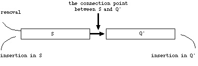 Figure 1 The
deque Q as a pair of stack (S) and queue (Q') (after Pallottino
1984, p.261).
Figure 1 The
deque Q as a pair of stack (S) and queue (Q') (after Pallottino
1984, p.261).
Because
a stack is used as a priority queue
in the PAP implementation, PAP has an exponential worst-case complexity
with respect to the number of nodes, i.e., O(n2^n). A logical
enhancement of the PAP algorithm is to replace the LIFO stack with a FIFO
queue and construct a new data structure. This new data structure
is called two-queue (Figure 2). Because both
Q' and Q" are queues in the two-queue data structure, nodes can be inserted
at the end of Q' and Q", and they can be removed from the head of
Q' and Q".
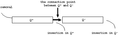 Figure 2 The
two-queue data structure (Q) consisting of Q" and Q' (after Pallottino
1984, p.264).
Figure 2 The
two-queue data structure (Q) consisting of Q" and Q' (after Pallottino
1984, p.264).
It follows
that for any node that is not already in Q, the node is inserted at the
end of Q' if it is unreached, or the node is inserted at the end of Q"
if it is temporarily labeled. This leads to the following change
in the Queue_Insertion(Q, j) operation of the PAP implementation (Pallottino
1984, p.264). Other operations remain the same.
Queue_Insertion(Q, j)
For any node j that is not already in Q,
insert the node at the end of Q' if the
node is unreached, i.e., if S(j) = unreached
or insert the node at the end of Q"
if the node is temporarily labeled.
5.
The Dijkstra's Algorithm Implemented With Approximate and Double Buckets
The original Dijkstra algorithm partitions all nodes into two sets:
temporarily and permanently labeled nodes. At each iteration, it
selects a temporarily labeled node with the minimum distance label as the
next node to be scanned (Dijkstra 1959; Ahuja et
al. 1993, p.109). Once a node is scanned, it becomes permanently
labeled. The Dijkstra algorithm terminates when all nodes become
permanently labeled. The Dijkstra algorithm is similar to the procedure
for constructing a shortest path tree described in Section 4 except for
the differences mentioned above. Therefore, detailed procedure of
the Dijkstra algorithm is not described further in this paper.
In Dijkstra's original algorithm,
temporarily labeled nodes are treated as a nonordered list. This
is equivalent to treating the priority queue Q in the above general procedure
for shortest path tree construction as a nonordered list. This is
of course a bottleneck operation because all nodes in Q have to be visited
at each iteration in order to select the node with the minimum distance
label. A natural enhancement of the original Dijkstra algorithm is
to maintain the labeled nodes in a data structure in such a way that the
nodes are sorted by distance labels. The bucket data structure is
just one of those structures. Buckets are sets arranged in a sorted fashion
(Figure 3). Bucket k stores all temporarily
labeled nodes whose distance labels fall within a certain range.
Nodes contained in each bucket can be represented with a doubly linked
list. A doubly linked list only requires O(1) time to complete an
operation in each distance update in the bucket data structure. These
operations include: 1) checking if a bucket is empty, 2) adding an element
to a bucket, and 3) deleting an element from a bucket.
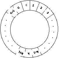 Figure 3
An example of the bucket data structure (after Ahuja
et al 1993, p.114).
Figure 3
An example of the bucket data structure (after Ahuja
et al 1993, p.114).
Dial
(1969) was the first to implement the Dijkstra algorithm using buckets.
In Dial's implementation, bucket k contains all temporarily labeled
nodes whose distance labels are equal to k. Buckets numbered
0, 1, 2, 3, ..., are checked sequentially until the first nonempty bucket
is identified. Each node contained in the first nonempty bucket has
the minimum distance label by definition. One by one, these nodes
with the minimum distance label become permanently labeled and are deleted
from the bucket during the scanning process. The position of a temporarily
labeled node in the buckets is updated accordingly when the distance label
of a node changes. For example, when the distance label of a temporarily
labeled node is changed from d(1) to d(2), this node is moved from bucket
d(1) to bucket d(2). This process is repeated until all nodes are
permanently labeled. Dial's original implementation of the Dijkstra
algorithm (DKB) requires nC+1 buckets in the worst case, where C
is the maximum arc length of a network. However, it has been proven
that for a network with a maximum arc length of C, only C+1
buckets are needed to maintain all temporarily labeled nodes (Ahuja
et al. 1993, pp.113-114).
It
can be seen that the memory requirement in DKB can be prohibitively large
when both C and n are large. However, the memory requirement
in DKB can be reduced using either the overflow bag implementation
(DKM) or the approximate buckets implementation (DKA) as described
by Cherkassky et al. (1993, p.7).
The overflow bag implementation maintains only a<(C+1) buckets
where a is an input parameter. Only temporarily labeled nodes
whose distance labels fall within the range of [a(i), a(i)+a-1]
are contained in the buckets at the i-th stage of the algorithm.
Other nodes are maintained in a separate set referred to as the overflow
bag. Initially, the values of i and a(i) are set
to 0. When there is no labeled node left in the given range,
i is incremented by one and a(i) is set equal to the minimum
of the distance label of the temporarily labeled nodes. The nodes
with distance labels within the new range of [a(i), a(i)+a-1]
are moved into their corresponding buckets from the overflow bag, and another
cycle of the scanning process begins.
The Dijkstra's algorithm
implemented with approximate buckets (DKA): In the approximate
bucket implementation of the Dijkstra algorithm (DKA), a bucket
i contains those temporarily labeled nodes with distance labels within
the range of [i*b, (i+1)* b-1], where
b is a chosen constant. Here approximate means that the values
of the distance labels in a bucket are not exactly the same as in the case
of DKB, but are within a certain range. Nodes in each bucket are
maintained in a FIFO queue. Algorithm DKA requires a total of largerInteger(C/b)+1
buckets. The worst case complexity of DKA is O(mb+n(b+C/b)).
It can be seen that this algorithm trades speed for space. Each node
can be scanned more than once, but a node cannot be scanned more than b
times.
The Dijkstra's algorithm
implemented with double buckets (DKD): The double bucket implementation
of the Dijkstra's algorithm (DKD) combines the ideas of the above two algorithms
DKM and DKA. Two levels of buckets, high-level and low-level, are
maintained in the DKD implementation. A total of d buckets
in the low-level buckets are used. A bucket i in the high-level
buckets contains all nodes whose distance labels are within the range of
[i*d, (i+1)* d-1]. In addition, a nonempty bucket with the
smallest index L is also maintained in the high-level buckets.
A low-level bucket d(j)-L*d maintains nodes whose distance labels
are within the range of [L*d, (L+1)* d-1]. Nodes in the low-level
buckets are examined during the scanning process. After all nodes
in the low-level buckets are scanned, the value of L is increased.
When the value of L increases, nodes in the nonempty high-level
buckets are moved to its corresponding low-level buckets, and the next
cycle of scanning process begins.
In recent years, we have witnessed an increasing popularity of transportation
related decision analysis within a GIS environment (see, e.g., Ralston
et al. 1994; Erkut 1996 and Noon et al. 1996). In this
type of analysis, the computation of shortest paths is often a central
task because shortest path distances are often needed as input for "higher
level" models in many transportation analysis problems such as facility
location, network flows, vehicle routing and product delivery, just to
name a few. In addition, the shortest path problem usually captures the
essential elements of more complicated transportation analysis problems.
Hence, it can often be used as a benchmark or a starting point for solving
more complicated problems in transportation analysis. With the advancement
of GIS technology and the availability of high quality road network data,
it is possible to conduct transportation analysis concerning large geographic
regions within a GIS environment. Sometimes, this type of analysis has
to be completed in real time. As a consequence, these analysis tasks demand
high performance shortest path algorithms that run fastest on real road
networks.
Although there has been
considerable reported research related to the evaluation of the performance
of shortest path algorithms, there has been no clear answer as to which
algorithm or a set of algorithms runs fastest on real road networks in
the literature. A recent evaluation of shortest path algorithms using real
road networks has identified a set of three algorithms that run fastest.
These three algorithms are: 1) The Graph Growth Algorithms implemented
with two queues (TQQ), 2) The Dijkstra's algorithm implemented with approximate
buckets (DKA), and 3) The Dijkstra's algorithm implemented with double
buckets (DKD). As a sequel to that earlier evaluation, this paper has reviewed
and summarized the data structures and procedures related to the three
algorithms. This paper provides a direct source that summarizes a set of
shortest path algorithms that run fastest on real road networks. This source
should be particularly useful for researchers and practitioners whose research
and practice are related to the use of shortest path algorithms.
Ahuja, R. K., Magnanti, T. L., and Orlin, J. B.(1993)
Network Flows: Theory, Algorithms and Applications. Englewood
Cliffs, NJ: Prentice Hall.
Ahuja, R. K., Mehlhorn, K., Orlin, J. B., and Tarjan, R. E. (1990)
Faster algorithms for the Shortest Path Problem. Journal of Association
of Computing Machinery, 37, 213-223.
Cherkassky, B. V., Goldberg, A. V., and Radzik, T. (1993)
Shortest Paths Algorithms: Theory and Experimental Evaluation.
Technical Report 93-1480, Computer Science Department, Stanford University.
Dial, R. B. (1969) Algorithm 360: Shortest Path Forest
with Topological Ordering. Communications of the ACM, 12,
632-633.
Dial, R. B., Glover, F., Karney, D., and Klingman, D. (1979)
A Computational Analysis of Alternative Algorithms and Labeling Techniques
for Finding Shortest Path Trees. Networks, 9, 215-248.
Dijkstra, E. W. (1959) A Note on Two Problems in Connection
with Graphs. Numeriche Mathematik, 1:269-271.
Erkut, E. (1996) The Road Not Taken. ORMS Today,
23, 22-28.
Gallo, G., and Pallottino, S. (1988) Shortest Paths Algorithms.
Annals of Operations Research, 13, 3-79.
Glover, F., Klingman, D., and Philips, N. (1985) A New
Polynomially Bounded Shortest Paths Algorithm. Operations Research,
33, 65-73.
Goldberg, A. V., and Radzik, T. (1993) A Heuristic Improvement
of the Bellman-Ford Algorithm. Applied Mathematics Letter,
6, 3-6.
Hung, M. H., and Divoky, J. J. (1988) A Computational Study
of Efficient Shortest Path Algorithms. Computers & Operations
Research, 15, 567-576.
Mondou, J.-F., Crainic, T. G., and Nguyen, S. (1991) Shortest
Path Algorithms: A Computational Study with the C Programming Language.
Computers & Operations Research, 18, 767-786.
Noon, C. E., Daly, M., and Zhan. F. B. (1996) Beyond Assessment
of Resources: Procurement of Woody Biomass Fuels. Proceedings of
Bioenergy'96 held in Nashville, Tennessee, pp.565-569.
Pallottino, S. (1984) Shortest-Path Methods: Complexity,
Interrelations and New Propositions. Networks, 14, 257-267.
Pape, U. (1974) Implementation and Efficiency of Moore
Algorithms for the Shortest Root Problem. Mathematical Programming,
7, 212-222.
Ralston, B., Tharakan, G., and Liu, C. (1994) A Spatial
Decision Support System for Transportation Policy Analysis. Journal
of Transport Geography, 2, 101-110
Sedgewick, R. (1990) Algorithms in C. Reading,
MA: Addison Wesley Publishing Company.
Zhan, F. B. (1995) Shortest Path Algorithms: Evaluation
and Implementation in C. Research Report. Department of Geography
and Planning, Southwest Texas State University, San Marcos, TX.
Zhan, F. B., and Noon, C. E. (1996) Shortest Path Algorithms:
An Evaluation Using Real Road Networks. Transportation Science
(in press).
 JGIDA
vol.1, no.1 JGIDA
Home
JGIDA
vol.1, no.1 JGIDA
Home
