Grégoire Dubois
Institute of Mineralogy &
Petrography, University of Lausanne, Switzerland
gregoire.dubois@usa.net
| Contents
1. Introduction 2. Nearest Neighbours Index (NNI) 3. Fractal dimension of sampling networks 4. Morisita Index 5. Thiessen/Voronoi polygons 6. Coefficient of Representativity (CR) 7. Conclusions References |
ABSTRACT
Sampling
schemes frequently present irregular structures that can affect the analyses
of the studied phenomenon. Many methods that can evaluate the sampling
bias do exist but none of them are entirely satisfying. These methods will
be briefly discussed here and on the basis of their advantages and drawbacks,
an attempt is made to design a new method which will evaluate the level
of "representativity" of samples in a monitoring network. This method introduces
a Coefficient of Representativity (CR) based on Thiessen polygons
as well as on distances of nearest neighbours. The use of this coefficient
should facilitate the identification of clustered data as well as isolated
points, allow the researcher to define the measurements that can be averaged
for declustering problems and make possible the comparison of different
sampling strategies for a given surface.
KEYWORDS: sampling network, spatial structure, coefficient of representativity, Morisita index, Thiessen/Voronoi polygons, fractals, nearest neighbours index. |
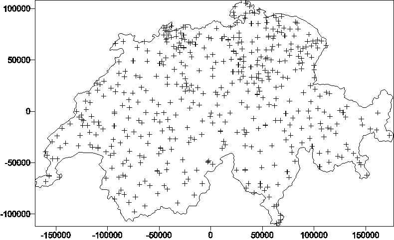
Figure 1. Sampling locations of the 467 measurements made in Switzerland |
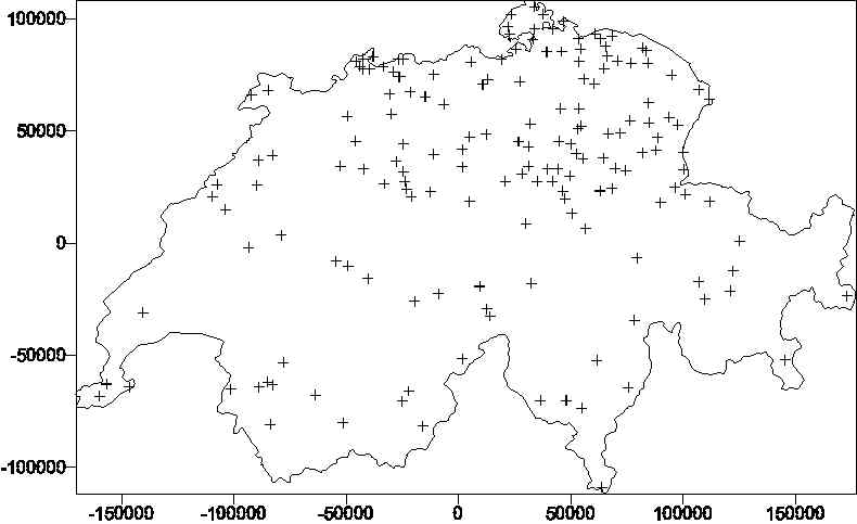
Figure 2. Subset of 167 samples from Figure 1. |
2.
Nearest Neighbours Index (NNI)
The nearest neighbours index (NNI) (Clark
and Evans, 1954) compares the distances between nearest samples to
distances that would be expected by chance. The NNI is defined as
the ratio of the mean of the Nearest Neighbours distances (NNdist),
that is
where N is the number of sampling points and, to the mean of the Nearest Neighbours distances for a uniform distribution of the points . This mean random distance (MRD) is defined as
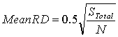
where Stotal is the total surface of the investigated area. The NNI is thus equal to
![]()
The NNI is close to 1 when the sampling points have an uniform
spatial distribution. When NNI < 1, the samples are more clustered
than expected compared to a random distribution. In the contrary, an NNI
> 1 indicates a dispersion of the samples. The statistics of the distances
to the nearest neighbours as well as the NNI are given in Table
1. The surface used as total surface is the area of Switzerland
(41 293 km2).
|
|
|
min(NN) |
|
|
|
| 167 points | 8.113 | 6.646 | 0.751 | 335.708 | 0.033 |
| 467 points |
5.641
|
2.433
|
0.751 |
335.708
|
0.038
|
One will note two limitations to the method. If the whole data set can be described by the NNI, it does not indicate the clusters. Secondly, the geometry of the analysed surface can be complex and have an impact on the spatial distribution of the sampling points.
3. Fractal dimension
of sampling networks
Mandelbrot (1982) introduced the term of "fractal"
which is used to describe continuous spatial phenomenon that present spatial
correlation at different scales. For a linear fractal function, the Hausdorff-Besicovitch
(D) dimension can vary between 1 (it can be completely derivated)
and 2, the function is so irregular that it covers the whole space of 2
dimensions. Lovejoy et al. (1986) have
applied fractals to describe de heterogeneity of measuring networks. When
the heterogeneity of the network appears at different scales of a space
of dimension E, it can be characterised by a fractal dimension Dm.
The authors have also shown that each time Dm< E,
phenomena of fractal dimension Dp < E - Dm
cannot be detected by the network even if the density of the monitoring
stations is infinite. Dm is defined by the variation
of the average number n(R) of observations found within a circle
with a varying radius R centered on each point of the monitoring
network. A set of measures has a fractal dimension Dm if
it satisfies the following condition
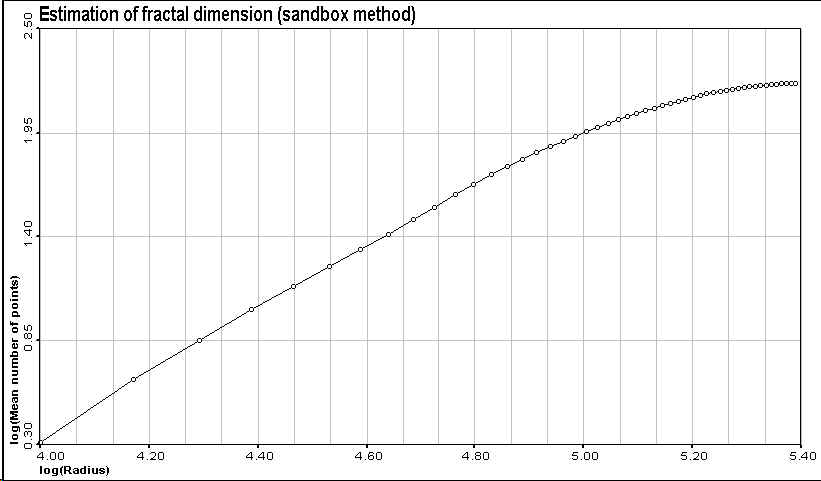
Figure 3. Estimation of the fractal dimension of the 467 points data set. |
|
The second one is due to border effects. The circle used to define the average number of points falling within R will find only a part of those found when the circle is somewhere in the middle of the data (Tessier et al., 1994 ; Doswell and Lasher-Trapp, 1997).
4. Morisita
Index
Another method is Morisita's Index (Morisita,
1959; Cressie, 1993, p. 578, 590-591). The analysed surface is divided
into rectangular cells of equal size d and the index is defined
as
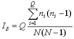 ,
,
where N is the number of points in the sampling network, ni is the number of samples found within the ith cell, and Q is the total number of cells. By displaying the values of the index against the size of the cells, one can investigate the degree of contagion of the sampling network, that is the probability that two points from the network fall within the same cell.
If the spatial distribution of the samples is random but homogeneous, Id is independent of the size of cells and fluctuates around a mean value of 1.
When clusters are present, Id becomes greater than 1.
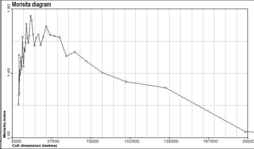
Figure 4. Morisita's diagram for the 467 points data set |
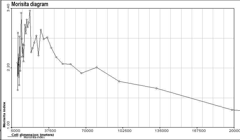
Figure 5. Morisita's diagram for the 167 points data set |
The maximum of the index, that is the typical size of a cluster, is reached for a cell size of 19 km for 467 points and 22 km for 167 points.
5.
Thiessen/Voronoi polygons
Thiessen polygons, also known as Voronoi polygons or Dirichlet cells
(Thiessen, 1911; Okabe et al., 1992) have
the property to contain only one measurement and to have a geometry that
will include all the data points that are closer to the measurement than
to any other measurement. Isolated observations will therefore have
polygons that will be larger than those associated to clustered data. These
polygons are also frequently used to define weights that are used to decluster
the data when an attempt is made to obtain statistics that are representative
of the studied phenomenon over the whole surface of interest (Isaaks
and Srivastava, 1989). Histograms of the areas of these polygons
might help to describe quantitatively the homogeneity of the sampling network:
by knowing the average cell size, which represents the cell size one would
have in case of an homogeneous network, one can evaluate the impact of
extreme values on the sampling network. The Thiessen polygons of the 467
points data set are shown in Figure 6.
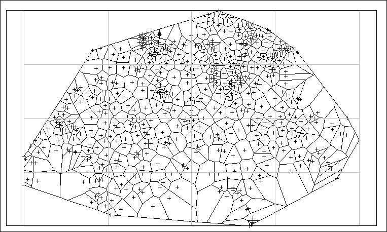
Figure 6. Thiessen polygons of the 467 sampling points. |

Figure 7. Frequency histogram of the surfaces of the Thiessen polygons shown in Figure 6. |
The frequency histogram of the surfaces of these
polygons (Figure 7) shows a skewed distribution: while
the ideal cell size, that is the total surface divided by the number of
samples, has a surface of 88.13 km2, one can observe few polygons
having extremely large areas and many small polygons highlighting the presence
of clustered data.
Two drawbacks appear when applying such a method.
The first one is due to the fact that the borders of the polygons are frequently
defined by a convex hull which is constructed on the basis
of the outern points. If such an approach is acceptable if one is working
only within the geographical limits defined by the sampling network, a
bias may be introduced when the shape of the analysed region does not correspond
to the convex hull. Geographic Information Systems (GIS) facilitate the
use of additional information that could better define the boundaries of
the region of interest. For the here presented case study, the sampling
network is expected to provide information for the whole surface of Switzerland.
Reconstructing the Thiessen polygons with the help of the country borders
will let appear a new map which is shown in Figure 8.
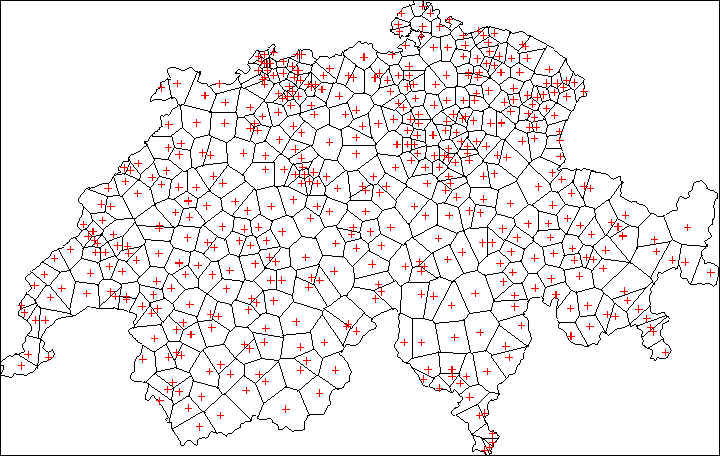
Figure 8. Thiessen/Voronoi polygons of the 467 sampling points and country borders. |
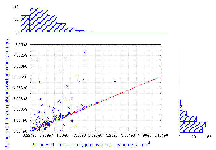 |
The differences between the surfaces of the Thiessen
polygons of the two maps (Figures 6 and 8)
are shown in Figure 9. The use of country borders has
clearly reduced the impact of the very large polygons found in the South
of the country .
A second problem in using such an approach is that points can be clustered
and still have relatively large Thiessen polygons as shown in Figure
10.
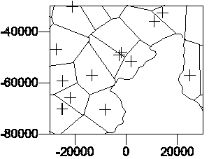
Figure 10. Large Thiessen polygons do not guarantee
that the points are isolated.
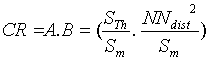
6.
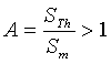
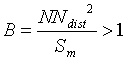
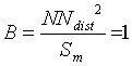
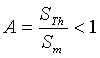
Coefficient of Representativity (CR)
One the basis of the preceding observations, a new measure that would
combine both the surfaces of Thiessen polygons and the distance of each
point to its nearest neighbour is proposed. This measure, which we will
call Coefficient of Representativity (CR), is a product of two terms:

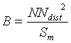
The properties of the CR are summarised in Table
3.
Table 3. Influence of parameter A (the area of the Thiessen polygon) and B (distance to Nearest Neighbour) on the coefficient of representativity (CR).
|
|
|
|
| Thiessen area > mean surface
|
NN > mean distance
|
CR > 1 |
| Thiessen area = mean surface
|
NN = mean distance
|
CR = 1 |
| Thiessen area < mean surface
|
NN < mean distance
|
CR < 1 |
Because a CR can be attributed to any sampling point, one can create maps of CR that should help to identify clustered data as well as regions where few data are available. For mapping purposes, one could use the logarithm of CR,
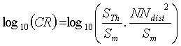 ,
,
instead of the CR so that the CR < 1 become negative. Figure 11 displays the values taken by log10(CR) for the 467 (top) and 167 (bottom) sampling points. Isolated points as well as those that are clustered are put in evidence, respectively by log10 (CR) > 0 and a log10 (CR) < 0.
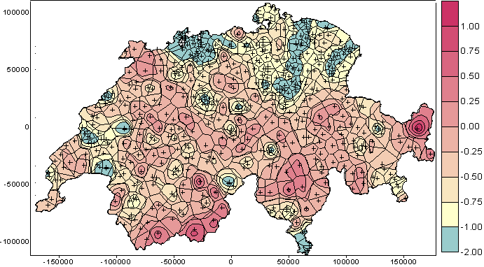
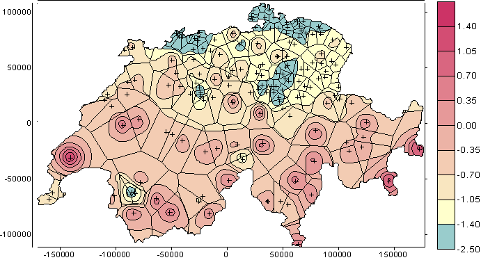
Figure 11. Levels of log10(CR) for 467 (top) and 167 (bottom) sampling points.
The mean, the standard deviation and the coefficient of variation (CV)
of the values taken by the CR also allow the description of the
structure of the sampling networks (Table 4).
|
|
|
|
|
| 167 points |
0.98
|
3.16
|
3.22
|
| 467 points |
0.63
|
1.29
|
2.05
|
CV's greater than
1 indicate the presence of high erratic values that underline the irregularity
of the sampling network. The CV for the 467 points data set is lower
than for 167 sampling points and shows therefore an improvement in the
spatial distribution of the sampling points even if clusters are still
present (the mean value of the CR is < 1). The proposed method
presents, however, a limitation. Points for which the CR = 1 (or
log10CR = 0) can not be automatically classified within
the class of those points that fall in the middle of Thiessen polygons
that have a surface that is equal to the expected average surface. A measurement
located within a large polygon but close to another point can indeed have
a CR = 1.
If the CR can not
be used directly to weight the samples prior to a declustering because
of the contagion problem, that is that two points very close to each other
will have a low CR, one can still make use of the CR's obtained
for each point for a declustering problem. The point that has the
lowest CR can be averaged to its nearest neighbour and a new sampling
network is obtained. By proceeding in such a way and after several
iterations, the CR of the network will tend to 1. A drawback is
that such a process can be time consuming since the construction of the
polygons has to be repeated after each iteration. Moreover, the use of
boundaries that have a complex geometrical shape might require from the
user to check to which polygons corresponds a single point since a single
polygon can be split in several pieces when "clipping" it with the boundaries.
The attempt to convert an irregular sampling network in a more regular
one is similar to triangulations techniques that fill the holes with points
until all triangles have the same sizes (Kanevsky
and Savelieva, 1995). The main difference comes from the averaging
of the data that will reduce systematically the amount of information while
preserving the most important one while the triangulation method requires
the sampling of new locations.
7. Conclusions
"All samples are equal but some are more equal than
others...". Isolated points require more attention than clustered data
even if these last ones are essential for the analysis of microscale variations
of the studied phenomenon. The Coefficient of Representativity should help
decision makers to improve sampling campaigns by identifying undersampled
areas as well as for the declustering of the data in order to obtain statistics
that are representative of the analysed phenomenon. One can argue that
the use of a single value to describe the complexity of sampling network
is somehow limitating. It does, however, allow the comparison of different
sampling strategies within a defined region. The CR benefits from
the information provided not only by both the NNI and the surfaces
of the Thiessen polygons, but also by the boundaries of the region of interest
which clearly influences the spatial structure of a monitoring network.
Used in combination with semivariograms, it should also provide an interesting
information on the impact of each sample during an estimation problem.
References
Burgess, T. M., R. Webster and A. B. McBratney (1981).
Optimal interpolation and isarithmic mapping of soil properties. IV. Sampling
strategy. Journal of Soil Science, 32: 643-659.
Burrough, P. A. (1991). Sampling Designs for Quantifying Map
Unit Composition. In Spatial Variabilities of Soils and Landforms,
Soil Science Society of America, SSSA Special Publication no. 28, pp. 89-125.
Clark, P. J. and F. C. Evans (1954). Distance to nearest
neighbor as a measure of spatial relationships in populations. Ecology,
35:
445-453.
Cressie, N. (1993). Statistics for spatial data. John
Wiley & Sons Inc., Revised Edition, 900 p.
Doswell III C. A. and S. Lasher-Trapp (1997). On measuring
the degree of irregularity in an observing network. Journal of Atmospheric
and Oceanic Technology, 14: 120-132.
Isaaks E. H. and Srivastava R. M. (1989). An introduction
to applied geostatistics. Oxford University Press.
Kanevsky M. and Savelieva E. (1995). Environmental monitoring
networks and quantitative description of clustering. In: Proceedings
of the annual conference of the International Association for Mathematical
Geology, IAMG, Osaka, Japan. pp. 31-32.
Lovejoy S., D. Schertzer and P. Ladoy (1986). Fractal
characterization of inhomogeneous geophysical measuring networks. Nature,
319: 43-44.
Mandelbrot, B. B. (1982). The fractal geometry of nature.
W.
H. Freeman.
Matheron G. (1963). Principles of geostatistics. Economical
Geology, 58: 1246-1266
McBratney, A. B., R. Webster and T. M. Burgess (1981). The design
of optimal sampling schemes for local estimation and mapping of ragionalized
variables. I. Theory and method. Computer & Geosciences 7(4):
331-334.
Morisita, M. (1959). Measuring of the dispersion and analysis
of distribution patterns. Memoires of the Faculty of Science, Kyushu
University, Series E. Biology. 2: 215-235.
Okabe A., B. Boots & K. Sugihara (1992). Spatial Tessellations.
Concept and Applications of Voronoi Diagrams. Wiley and Sons.
Oliver M. A. and Webster R. (1986). Combining nested and
linear sampling for determining the scale and form of spatial variation
of regionalized variables. Geographical Analysis, 18(3): 227-242.
Tessier Y., S. Lovejoy and D. Schertzer (1994). Multifractal
analysis and simulation of the global meteorological network. Journal
of Applied Meteorology, 33: 1572-1586.
Thiessen, A. H. (1911). Precipitation average for large areas.
Monthly
Weather Review, 39: 1082-1084.