Journal
of Geographic Information and Decision Analysis, vol. 4, no. 1, pp. 11-28
Local Machine Learning Models
for Spatial Data Analysis
Nicolas Gilardi
Mineralogy Institute, University
of Lausanne, Switzerland
gilardi@idiap.ch
Samy Bengio
IDIAP, Martigny, Switzerland
bengio@idiap.ch
http://www.idiap.ch/~bengio
Contents
1.
Introduction
2.
Global Models
2.1
Support Vector Regression
2.2
Multilayer Perceptrons
3.
Local Models
3.1
Local SVR
3.2
Mixture of Experts
3.3
Local Models and Geostatistics
4.
Model Selection
5.
Case Study
5.1 Dataset
5.2
Experimental Setup
5.3
Results
5.4
Beyond SIC97
6.
Conclusions
References |
ABSTRACT
In
this paper, we compare different machine learning algorithms applied to
non stationary spatial data analysis. We show that models taking into account
local variability of the data are better than models which are trained
globally on the whole dataset. Two global models (Support Vector Regression
and Multilayer Perceptrons) and two local models (a local version of Support
Vector Regression and Mixture of Experts) were compared over the Spatial
Interpolation Comparison 97 (SIC97) dataset, and the results are presented
and compared to previous results obtained on the same dataset.
KEYWORDS:
machine
learning, multilayer perceptron, neural networks, support vector machine,
support vector regression, mixture of experts, non-stationarity, SIC97,
local model. |
During the last decade, machine learning algorithms, such as artificial
neural networks, have been extensively used for a wide range of applications.
They have been applied for classification, regression, and density estimation
tasks (see (Bishop 1995) for a good overview).
In fact, many fields of research using feature extraction or data prediction
(and there are many) have been trying some machine learning models, with
more or less success. Analysis of spatial data has been involving these
methods as well, like in (Kanevksi
et al. 1996) and (De Bollivier
et al. 1997), but such ideas are not so much exploited for what concerns
Geostatistical data.
One possible reason to this
can be the ``black box'' aspect of most of these algorithms. Tuning them
can be very difficult and without a clear methodology and some prior information
about data, it can often lead to bad results. Another reason is that the
tuning of most learning algorithms is partly based on theoretical machine
learning arguments and rarely on some expertise on the problem to solve,
and thus difficult to interpret. Therefore, it can appear unnecessary to
use such complex methods when one have more simple but yet efficient one.
However when the simple methods can no longer be applied due to the complexity
of the data, these machine learning algorithms have to be considered in
order to expect better results at the price of loosing some interpretability
of the underlying models.
In this paper, we try to
demonstrate the potential of machine learning algorithms, showing that
a specific adaptation to the given problem of two basic learning methods,
multilayer perceptron and support vector regression, can improve significantly
their performances on a given dataset. One of these adaptations (mixture
of experts) is a direct usage of an existing machine learning algorithm,
and the other one (local support vector regression) is a modification of
the training procedure of the original algorithm, using Geostatistical
a
priori knowledge, in a similar way than it has been done by De Bollivier
et
al for local multilayer perceptron (De
Bollivier et al. 1997).
In the following two sections,
we introduce the methods compared in this paper, first the global methods
(support vector regression and multilayer perceptron), and then the local
methods (local support vector regression and mixture of experts). The next
section is then devoted to the methodology we used in order to select the
values of the hyper-parameters of all machine learning algorithms in order
to avoid any bias. Finally, in the experimental section, we apply all these
methods to the Spatial Interpolation Comparison 97 (Dubois
et al. 1998) dataset, and compare and comment the results.

|
Figure 1: SVR linear regression
with  -insensitive
loss function.
Directly derived from Vapnik and Chervonenkis'
Statistical Learning
Theory (Vapnik 1995), Support
Vector Machines (SVM) for classification problems were developed during
the beginning of the 90's (a good overview of SVMs can be found in
(Burges 1998)). Later, the algorithm
was extended to deal with regression problems. This new algorithm was thus
named Support Vector Regression (SVR) (Smola
et al. 1998), and we present it here briefly.
For a given set of data  ,
,  and
and  ,
the simplest linear SVR algorithm tries to find the function
 minimizing the quadratic optimization problem

where, in our case  corresponds to Vapnik's
  -insensitive
loss function, which does not penalize errors less than
  (cf. figure 1). After some reformulation
and taking into account the case of non-linear regression, the optimization
problem is then transformed into the minimization of

subject to
 where the
  are Lagrange multipliers, solutions of the optimization problem, C
is the soft margin parameter, weighting the influence of the loss
function against the regularization term, and k(xi,xj)
is a kernel function, defining the feature space in which the optimal
solution of the problem will be computed in order to handle non-linear
problems. In our experiments, we used the Gaussian Radial Basis Function
(RBF) kernel:

To estimate a new point, we then use the following function f:

where the  are the indices of the data points for which either
  or
or  is non zero. Those points are called support vectors (red points
in Figure 1).
|
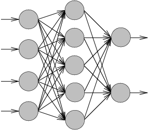
Figure 2: The architecture of
an MLP.
A multilayer perceptron (MLP) is a particular architecture of artificial
neural networks, composed of layers of non-linear but differentiable parametric
functions. For instance, Figure 2 shows an
MLP with one input layer of size 4, one hidden layer of size 5 and one
output layer of size 2. Alternatively, an MLP can be written mathematically
as follows:

where the estimated output  is a function of the input vector x
(indexed by its M values xm), and the parameters
 ![$\{\theta: w_n, w_{nm}, b_n, b; \mbox{ with } n \in [1,N],m \in [1,M]\}$](img21.gif) .
This MLP is thus a weighted combination of N hyperbolic tangents of weighted
combinations of the input vector. Given a criterion Q to minimize,
such as the mean squared error,
.
This MLP is thus a weighted combination of N hyperbolic tangents of weighted
combinations of the input vector. Given a criterion Q to minimize,
such as the mean squared error,

between the desired output yi and the estimated output  ,
for a given training set of size l, one can minimize such criterion
using a gradient descent algorithm (Rumelhart
et al. 1986). This algorithm is based on the computation of the partial
derivative
  of the criterion Q with respect to all the parameters
  of
of  .
The gradient descent can then be performed using

for each parameter  where
where  is the learning rate. It has been shown that given a number of hyperbolic
tangents N sufficiently large, one can approximate any continuous
function using such MLPs (Hornik et al.
1989).
As proposed by Bottou and Vapnik in (Bottou
et al. 1992), when the data is clearly non-evenly distributed, one
can significantly improve the prediction results of machine learning algorithms
by building multiple local models instead of one global model. In this
section, we propose the use of two local methods, based respectively on
SVRs and MLPs.
The proposed algorithm builds one SVR model for each point to be estimated,
taking into account only a subset of the training points. This subset is
chosen on the basis of the Euclidean distance between the testing point
and the training point in the input space. For each testing point, a new
SVR model is thus learned using only the training points lying inside a
user defined radius which center is the current testing point.
The radius can be chosen
in relation to the a priori spatial correlation of the data, or
like any other hyper-parameters, i.e. by cross-validation (see Section
4 for an introduction to cross-validation). It is also possible to
use an anisotropic neighborhood, for example an ellipsoïd, instead
of a circle. With such a point selection, one can ``force'' the local model
to adapt itself to an anisotropic phenomenon.
A problem related to local
SVR estimation (besides the computational time needed to create all these
local models) concerns the number of points in the subset. If the selected
radius is too small, it might happen that some testing points will have
a very small number of training points in their subset (or even none).
Theoretically, the SVR algorithm can work even with only two training points
(with input vectors in two dimensions). But due to numerical stability
of the optimization, it is better not to estimate any SVR model with less
than four training points. Testing points in this situation can thus be
estimated by simple mean value or inverse distance, which would not be
very different from what SVR would have predicted on such a small number
of point.
On the contrary, if the
research radius is large, one might have a very large number of training
points, which can lead to long training time, considering the fact that
we are computing one model for each testing point! Thus, in order to speed
up the procedure, one might consider to limit the number of training points
taken into consideration. It is also important to note that testing points
very close to each other will probably have the same neighbors in the training
set, and thus, only one model should be necessary to predict those testing
points.
|
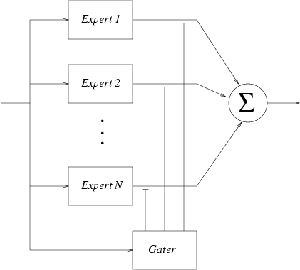
Figure 3: The architecture of
a mixture of experts.
A mixture of experts (Jacobs et al.
1991) is a very simple model that embodies the divide-and-conquer principle:
instead of trying to fit a unique model for a whole training set, one supposes
that dividing the training set into many smaller training sets could simplify
the problem. The idea of a mixture of experts is then to simultaneously
(a) learn a soft division of the training set into different parts1
and (b) learn a different model on each part. As shown if Figure
3, in its simplest form, a mixture of experts is thus composed of N
modules, each receiving the same inputs, and each trying to output the
desired target. An additional module, the gater, also receives the
same input but has Noutputs which corresponds to the probability
of each module to give the correct target. It thus computes a soft partition
of the input space. More formally, for each input/output point (xi,yi),
each model mn is computing E(yi|xi,mn)the
expectation of the output yi given the input xi,
and the gater is computing P(mn|xi)
the probability of model mn given the input xi.
The overall output of the mixture of experts is then

with the constraint that

In the particular case where the gater and the models are represented
by differentiable parametric functions such as multilayer perceptrons2,
the whole system can be optimized jointly by minimizing an overall criterion
Q
such as the mean squared error over the whole training set. For parameters  of a given model mn, the derivative of the criterion
with respect to the parameters is as follows

and for parameters  of the gater, the derivative is as follows

Finally, it is important to note that one does not have to decide the
partition of the training set but still has to decide the number of such
partitions. This can be done using for instance a cross-validation technique,
as described in Section 4 on Model
Selection.
As Geostatistical data are often influenced by various local phenomena,
the idea of using local models applied to Geostatistical problems was also
developed for classical Geostatistical interpolation methods, like ordinary
kriging (Haas 1990) as well as with
MLPs (De Bollivier et al. 1997).
In the latter however, the authors do not use mixture of experts but instead
they propose to use MLPs trained using local data, in a similar way as
we proposed to use local SVRs.
Most of the models proposed in the machine learning literature, and all
the models proposed in this paper, have some hyper-parameters that
need to be selected prior to learning. Hyper-parameters are parameters
of the algorithm that are defined by the user and which influence the training
procedure. For instance, for an iterative algorithm, it could be the number
of iterations; for a multilayer perceptron, it could be the number of hidden
units; for a support vector machine, it could be a parameter related to
the chosen kernel; in fact, most of the models usually have more than one
hyper-parameter. In order to select them appropriately, some kind of hyper-learning
method is needed.
The method depends on the
size of the dataset. When it is large enough (usually more than a few thousand
examples), a simple method works as follows:
-
Randomly divide the dataset into two parts, a training set and a
validation
set (the validation set is usually smaller than the training set, depending
on the total size of the dataset).
-
For each value of the hyper-parameter (if there is more than one hyper-parameter
then, for each set of values of the hyper-parameters), train a model on
the training set and compute the performance of the trained model
on the validation set.
-
Select the value of the hyper-parameter that produced the model that gave
the best performance on the validation set and train the corresponding
model with the whole dataset.
The main idea behind this method is that the hyper-parameters have to be
chosen with data that were not used for training in order to avoid any
bias. However, when the size of the dataset is too small, which is often
the case in Geostatistical problems, this simple method becomes too noisy
and depends strongly on the arbitrary division between the training and
the validation sets. An extension of this method, called cross-validation,
and which have many variants, should then be used. For the current study,
we used the K-fold cross-validation method:
-
For each value of the hyper-parameter (if there is more than one hyper-parameter
then, for each set of values of the hyper-parameters), estimate the generalization
performance of the corresponding model as follows:
-
Randomly divide the dataset into K partitions of approximately the
same size.
-
For each partition, train a model using the data from the K-1 other
partitions and compute the generalization performance of all the examples
of this partition.
-
Add all generalization performances to compute the overall generalization
performance of the model with the current value of the hyper-parameter.
-
Select the value of the hyper-parameter that produced the model that gave
the best generalization performance and train the corresponding model with
the whole dataset.
Note that these methods do not give a good estimate of the performance
of the selected model on new data since all the examples have been used
to select the model. When one wants also to estimate the generalization
performance of the selected model, one needs to do two embedded cross-validations:
one to select the right model and one to estimate its performance. In the
current study, we did not estimate the generalization performance since
the goal was to select a model and then give predictions on a separate
dataset.
 |
 |
| (a) Training Set |
(b) Testing Set |
Figure 4: SIC97 training and
testing datasets. The training set consists in 100 rainfall measurements
in 1/10th of millimeters. The testing set consist in 367 measurement locations
where rainfall must be predicted. The true values in 1/10th of millimeters
are presented here.
The dataset we used to compare local and global machine learning methods
is the same as the one used in the Spatial Interpolation Comparison 97
(SIC97) (Dubois et al. 1998). It consists
in 467 daily rainfall measurements made in Switzerland, splited into a
training set of 100 points and a testing set of 367 points (Figure
4). Given the training set and a digital elevation model, SIC97 participants
had to predict rainfall at the 367 locations of the testing set.
The SIC97 dataset is characterized
by the small amount of training data and by a second order non-stationarity,
which means that correlation between data values is not independent from
data position, which is a sign of local phenomena. Another interesting
challenge in the use of such a dataset is that the training set distribution
is slightly different from the whole dataset, information which was provided
only a posteriori to the participants of the competition. Finally,
a lot of contributions exists (Dubois
et al. 1998), from which only a few were based on machine learning
algorithms. It is thus a good benchmark to compare methods.
In all experiments, only X and Y coordinates were used as input information.
Experiments using also altitude did not improve significantly the results
of the first model tried (the global SVR), and so, for a better comparison,
it has not been used for the other models (but it might be done in a close
future).
The choice of the hyper-parameters
was done by K-fold cross-validation on the training data, inside a user
defined set of hyper-parameters. Such an approach can become very time
consuming when the number of hyper-parameters is high. It is therefore
necessary to restrict the range in which these values should be selected.
5.2.1
Global SVR
The kernel parameter  ,
which is the standard deviation of a Gaussian function, is directly related
to the local variability of the data: the more the data is locally variable,
the smaller it should be. In practice, it is of no use to compute a model
with a value of
  greater than half the maximum distance between our data points: choosing
such a high value would imply a very low variability and thus no significant
improvement would rise from increasing the
  value. Following the same idea,
  cannot be smaller than half the smallest distance between the training
points: this would imply a variability so high that no prediction would
be possible as data points would be too far from each other (with respect
to the Gaussian) to extract any correlation information.
The precision parameter  has also an upper bound. It should not reach the difference between the
highest and the smallest output values of the training set. If so, there
would be no data points to compute the model, as they would all be considered
as ``acceptable mistakes''. By the way, this upper bound is far too high
in many cases. In Kanevski et al.
(2000),
  value is said to be upper-bounded by the value of the local variability
of the data, the so called ``nugget level'' of the semi-variogram3.
In SIC97 data, the nugget effect is almost zero, so the optimal
  value should be very small with respect to data value, and a range from
0 to 50 was thus chosen.
The soft margin parameter
C
is much more difficult to limit. It is related to the confidence we have
in our data: the highest it is, the more we believe in the training data.
This hyper-parameter is unlimited, so usually, one gives it various powers
of 10 in order to find the optimal one, but it might not be the most efficient
method.
5.2.2
Local SVR
 |
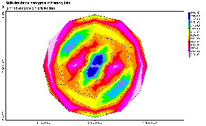
Figure 5: Multi-directional
variogram of training dataset. The anisotropy of spatial correlation is
clearly visible and can be used to improve the efficiency of prediction
models.
For the local SVR, one has to define the search neighborhood, in addition
to the other SVR hyper-parameters. This neighborhood was chosen with respect
to the range and the anisotropy given by the semi-variogram of the whole
training set (Figure 5). Of course, it
might looks strange to use global parameters to compute local models. But
due to the small number of data available, a computation of local semi-variograms
would have been noisy and thus irrelevant. Moreover, a local adjustment
of the anisotropic parameter would have been far too expensive in terms
of computation time. Thus, the most important to extract the local correlation
is to focus mainly on the first lags of the variogram, which are more likely
to be related to the local correlation.
5.2.3
MLP
For the multilayer perceptrons, we had to select the number of hidden units
(N), the number of learning iterations, and the value of the learning
rate ( ).
In fact, instead of using a simple gradient descent method, we used a conjugate
gradient method, which takes into account second order information and
do not need to select a learning rate
  .
All these hyper-parameters are related to the
capacity of the learning
system: the more examples one have, the higher the values of the hyper-parameters
could be, but their optimal value are problem dependent and can only be
chosen by cross-validation. Some simple rule of thumb still exists, such
as the fact that the number of parameters (weights and bias), which is
related to the number of hidden units, is usually smaller than the number
of training examples. But these rules of thumb should be used carefully,
only to give an idea on the range of the values to select with cross-validation.
The number of hidden units was thus chosen in a range from 5 to 40 and
the number of iterations was chosen in a range from 100 to 1000.
5.2.4
Mixture of Experts
For the mixture of experts, we had to decide the number of experts and
how to represent the experts and the gater. We decided to put most of the
capacity
into the gater so we represented it by an MLP, with various number of hidden
units (from 5 to 40). The experts were then represented by simple linear
models (weighted combinations of the inputs). The number of experts is
not easy to select. It should reflect the non-stationarity of the data,
but it should also take into account the total number of examples in the
training set. Therefore, we chose it in a range from 2 to 12. Finally,
the number of iterations was chosen in the same manner as for the MLP experiments.
5.3.1
Visual Results
 |
 |
| (a) Global SVR predictions |
(b) Local SVR predictions |
 |
 |
| (c) MLP predictions |
(d) Mixture of experts predictions |
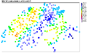
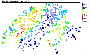
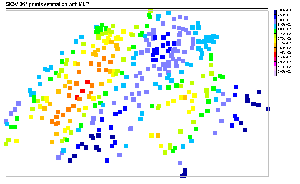
Figure 6: Estimations of SIC97
testing data with various machine learning models. The color scale is the
same for all pictures and corresponds to the one of Figure
4.
Figure 6 is a visual comparison of
SIC97 testing dataset predictions. Each of the four machine learning models
studied is represented here. All the models did reproduce the large anisotropy
of the SIC97 dataset, and the general predictions are quite close to the
original data, with a large band of low precipitation from South-West to
North-East, surrounded by two medium-to-high precipitation areas. The most
visible difference between each model concerns the estimation of the extreme
values. The global SVR failed in this task: the main tendencies are recovered,
but the final result seems to be too smooth. The local SVR performs better
in predicting high values and some very local phenomenon (like the ``hot
spot'' in the West), but a large band of high rainfall is under-estimated.
The MLP seems to perform better in the prediction of this high values band,
but the North-West frontier is underestimated, as well as the hot spot
detected by the local SVR. For the mixture of experts, the whole high precipitation
region is predicted with a very good efficiency, and despite some difficulties
in the North-West frontier, the general results seems to be the best of
all four.
 |
 |
| (a) Global SVR errors |
(b) Local SVR errors |
 |
 |
| (c) MLP errors |
(d) Mixture of experts errors |
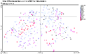
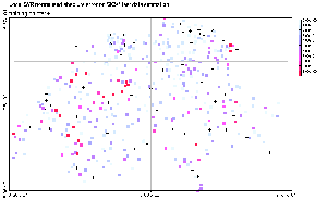
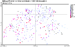
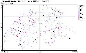
Figure 7: Normalized Absolute
error of SIC97 testing data predictions. The normalized absolute error
corresponds to the absolute error made by the predicting model at each
location, divided by standard deviation of the whole SIC97 dataset (train
+ test). The position of the training points is represented by crosses.
A
better overview of all this appears in Figure
7, which presents the normalized absolute prediction error made by
each model. A first overview shows that the two global models are overall
making higher errors than the two local models. Especially, the global
SVR seems to fail in all extreme value predictions, while the MLP gives
poor predictions in the North-West border. The local SVR and the mixture
of experts are both significantly improving the performance of their global
counterpart.
5.3.2
Spatial Correlation
 |
 |
| (a) Variograms of estimations |
(b) Variograms of residuals |
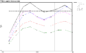
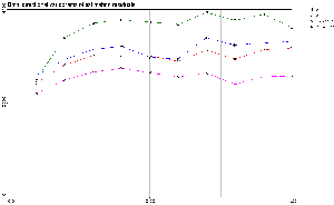
Figure 8: Omni-directional semi-variograms
of SIC97 testing data estimations and residuals. The left figure shows
the variograms from the four estimations, compared to the ``true'' one
and to the a priori variance of the testing data. The right figure
shows the variograms of the residuals of the four predictions, confronted
to each other, in order to compare the remaining correlation inside error
maps.
In Figure 8, one can compare the omni-directional
semi-variogram of the original testing data to the ones obtained by the
machine learning model estimations. It is interesting to notice that every
four models managed to reproduce the general spatial correlation quite
well over a large distance (the MLP is a bit worse at very large distance,
but this is not really important). However, the global SVR estimation is
very smooth, as the reduction of variance attests. This aspect of smoothing
is also present for the local SVR, but the improvement with respect to
the global SVR is quite significant. The MLP and the mixture of experts
outperform both, reproducing almost exactly the rise of the short range
correlation.
The variography of estimation
residuals gives also some information about the feature extraction quality
of each models for the SIC97 data. Thus, one can notice that the global
SVR did not manage to extract all information, as residuals appears to
be strongly correlated. But even if the remaining correlation is not as
high, it exists also for the other methods, showing that some improvement
is still theoretically possible. It is finally interesting to see that
local models have improved the feature extraction capabilities of the global
ones.
5.3.3
Numerical Results
Table 1 presents the numerical results of
global and local model predictions of SIC97 testing dataset. In addition
to root mean square error (RMSE) and mean absolute error (MAE), comparisons
to the real SIC97 testing data statistics is also presented. The last part
of the table summarizes the results of SIC97 as presented in (Dubois
2000). ``SIC97 best'' and ``SIC97 worst'' gives the corresponding results,
in terms of absolute deviation to the real value, found by the submitted
models for this specific table section (i.e. the best RMSE and the best
MAE do not correspond to the same model). ``SIC97 median'' gives the interval
inside which the statistics of the best 50% of the submitted models are.
Table 1: Comparison of multiple models over
SIC97 dataset. The models compared were multilayer perceptrons (MLP), Support
Vector Regression (SVR), mixture of experts (ME), and local SVR. They were
compared to the best, median and worst results for the SIC97 competition.
Results are given in terms of root mean squared errors (RMSE), mean absolute
error (MAE), as well as some statistics such as the minimum predicted value
(MIN), the median (MEDIAN), the maximum (MAX), the mean (MEAN) and the
standard deviation (STDEV).
| |
RMSE |
MAE |
MIN |
MEDIAN |
MAX |
MEAN |
STDEV |
| SIC97 true |
N.A. |
N.A. |
0 |
162 |
517 |
185 |
111 |
| MLP |
59 |
45.8 |
8.9 |
186.9 |
380.6 |
188.2 |
96.5 |
| SVR |
63.4 |
45.9 |
37.5 |
165.6 |
369.6 |
184 |
77.1 |
| ME |
53.2 |
38.6 |
0 |
165.3 |
453.8 |
182.5 |
101.7 |
| Local SVR |
57.1 |
41.9 |
0 |
163 |
472.7 |
182 |
88.8 |
| SIC97 best |
53.1 |
32 |
0 |
162 |
514 |
185 |
111 |
| SIC97 median |
63 |
44 |
[-15.5;15.5] |
[154;170] |
[462.5;571.5] |
[181;189] |
[99;123] |
| SIC97 worst |
99 |
70.6 |
-413 |
191 |
788 |
159 |
139.5 |
|
The numerical results give some
complementary details compared to the pictures. First of all, we have a
clear confirmation that, in terms of RMSE and MAE, local machine learning
models perform better on SIC97 data than global ones. In addition, they
are also able to reproduce quite efficiently the general statistics of
the data, which can be interpreted as a good estimation of the probability
density of the dataset. This second aspect is particularly true for the
local SVR. Compared to the MLP in terms of RMSE, these models are not significantly
different4,
but when looking at general statistics, the local SVR is always better
than the MLP, except for standard deviation conservation, as already shown
in Figure 8.
Comparing now the results
of the models to the general results from SIC97 contributions, one can
notice first that all the machine learning algorithms presented here are
at least as good as 50% of the methods published in 1998. Notice also that
global models are worse to predict high extreme values (MAX < 462.5),
and that SVR models have some difficulties to recover the variability of
the data (STDEV < 99). Finally, the mixture of expert results appear
to be one of the best published in terms of RMSE.
5.3.4
Conclusion on SIC97 Experiments
SIC97 benchmark, due to its complexity, has risen some drawbacks of global
machine learning algorithms for Geostatistical data. While these methods
were able to be almost as good as other regression techniques, they were
less efficient than most model based approaches, like ordinary kriging.
Various explanations can be formulated to explain this, but we can summarize
them into the problem of quantity of information. As they are model free,
learning algorithms are very sensitive to ``bad'' datasets. If the dataset
is small and/or noisy, its probability distribution can be very far from
the true probability distribution of the phenomenon. And without
a priori
knowledge, it becomes impossible to a learning algorithm to solve such
problem efficiently. When used by experimented users, model based methods
are often less sensitive to data representativity because the model becomes
user's prior information about the phenomenon.
To limit these problems,
we have chosen to build models focusing on local phenomena. In the case
of the local SVR, we used some specific knowledge we had on data (such
as spatial correlation and anisotropy) to artificially specialize the algorithm.
Results are good as the improvement on all criteria is significant, with
respect to the global SVR approach. The mixture of experts do not use more
a
priori knowledge than the underlying idea that one should focus on
some local phenomena. And it is keeping some global information as it is
building various global models locally weighted. As a consequence, it is
able to extract phenomena to a larger scale than the local SVR (which is
limited by its search neighborhood), with thus a better prediction ratio,
but generates a smoother structure (although more variable globally).
Beyond the quantitative results of the Spatial Interpolation Comparison,
it is interesting also to build some ``precise'' map of prediction of our
models. Of course, it will be impossible then, to say quantitatively whether
a model is better than another. But sometimes, a visual result is emphasizing
some interesting details otherwise unseen by plain general statistical
information, which is only a summary of a phenomenon.
5.4.1
Prediction on a Dense Grid
 |
 |
| (a) Global SVR predictions |
(b) Local SVR predictions |
 |
 |
| (c) MLP predictions |
(d) Mixture of experts predictions |
Figure 9: Prediction of a dense
grid of 47871 points using the four models used for SIC97 data estimation.
Color scale is similar to the one used for SIC97 estimation maps.
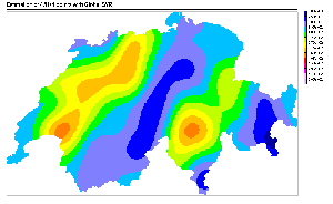
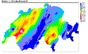
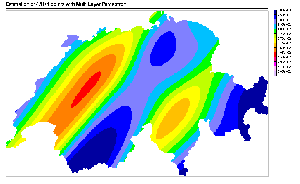
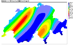
Figure 9 shows the prediction of the models
on a dense grid of 47871 points. The difference between models predictions
are impressive. First of all, one notices immediately the big difference
between the global SVR, the MLP and the mixture of experts maps compared
to the local SVR one. While the formers have a very regular and smooth
behavior, the latter is very sharp and complex. This behavior is a direct
consequence of the local modeling of the local SVR method. While the global
SVR and the MLP are using one model for all predictions, and the mixture
of experts is using a linear combination of a small number of them, the
local SVR approach is using, in the present estimation, around 2000 models
applied to very specific regions. The absence of overlapping between the
models explains the numerous discontinuity in the picture, and the local
spots are a result of the different optimal hyper-parameters found during
the training procedure. Finally, the strong anisotropy imposed to the training
procedure is very easy to identify. Too easy to be realistic, in fact.
Even less realistic for
a rainfall map are the other three pictures. The global SVR one has the
characteristic round-shape behavior of radial basis functions. These shapes
are very different from the one given by the MLP, closer to an ellipsoïde.
The mixture of experts structure is quite similar to the MLP's. It can
appear a bit strange that the mixture of experts has a so simple structure
whereas it has a multiple model structure; but this model is based on a
combination of a small number of linear models, and thus, the visual complexity
of the final prediction stays quite low.
The range of variation of
the data is also worth to be noticed. The global SVR is unable to generate
extreme values for its prediction while the other methods are. The local
SVR is even able to reach very high values on specific hot spots, while
the MLP and the mixture of experts are able to predict those high and low
values over large areas.
5.4.2
Omni-Directional Variograms of Dense Grid Estimations
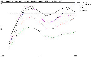 |
Figure 10: Omni-directional
semi-variogram of large grid prediction. The variograms of the four models
used to predict the 47871 grid points are represented with the SIC97 data
variogram for comparison.
The direct consequence of
this variability is represented in the omni-directional variograms shown
on Figure 10. The general behavior is very
similar to the one of Figure 8. The only
difference is that the overall variability of the data has increased. The
most surprising with these curves is that one could expect that, given
the very sharp and complex picture generated by the local SVR model, its
variogram would have been ``higher'' (i.e. more variable) than the ones
from the other models generating smooth and regular pictures. And interestingly,
this is not the case. The reason is that the local SVR is generating fewer
extreme values than the mixture of experts or the MLP and thus, the ``long''
range variability is smaller. The sharpness of the local SVR picture, opposed
to the smoothness of the other methods, is visible on the nugget effect:
the local SVR's one is higher than for all the other methods, sign of a
higher local variability.
The conclusion one can extract
from this qualitative comparison is that none of the studied regression
models is able to give a realistic behavior of the studied phenomenon.
The mixture of experts, the MLP and the global SVR are too smooth, while
the local SVR produces discontinuous and highly anisotropic features. Thus,
it is necessary to remember that predictions done using machine learning
methods, like with any other method, are strongly correlated to the method
used. And usually, learning algorithms are focusing more on minimizing
general statistics (like the expected mean squared error) than local variances,
except when trained to do so.
As it has already been experimentally shown in the Machine Learning and
Geostatistical fields (among others), local models perform usually better
than global ones on non-stationary datasets. The experiments conducted
on SIC97 data not only reflect the sensitivity of machine learning methods
to small and non representative datasets, but also proves that these methods
can be efficiently adapted to deal with such problems, and then give better
results.
Further researches are now
necessary to build some new machine learning methods, specifically adapted
to solve Geostatistical problems when classical methods are unable to do
so. Mixture models seems to be an interesting direction to follow in order
to complete this task. As far as the Support Vector Machines is concerned,
it seems that this algorithm is more efficient to solve classification
tasks than regression one, although kernel methods appear to be more interpretable
than multilayer perceptron.
-
1
-
Bishop, C. (1995)
Neural Networks for Pattern Recognition.
Clarendon Press, Oxford, 1995.
-
2
-
Bottou, L., and Vapnik, V. (1992)
Local learning algorithms.
Neural Computation, 4:888-900, 1992.
-
3
-
Burges, C.J.C. (1998)
A tutorial on support vector machines for pattern recognition.
Data Mining and Knowledge Discovery, 2(2):1-47, 1998.
-
4
-
De Bollivier, M., Dubois, G., Maignan, M., and Kanevski, M. (1997)
Modified multilayer perceptron with local constraint: Artificial neural
networks as an emerging method in spatial data analysis.
Nuclear Instruments and Methods in Physics Research, A389:226-229,
1997.
-
5
-
Dubois, G. (2000)
Intégration de système d'information géographique
et de méthodes géostatistiques.
PhD thesis, University of Lausanne, 2000.
-
6
-
Dubois, G., Malczewski, J., and De Cort, M. (1998)
Spatial interpolation comparison 97.
Journal of Geographic Information and Decision Analysis, 2(2),
1998.
Special issue.
-
7
-
Haas, T.C. (1990)
Kriging and automated variogram modeling within a moving window.
Atmospheric Environment, 24A:1759-1769, 1990.
-
8
-
Hornik, K., Stinchcombe, M., and White, H. (1989)
Multilayer feedforward networks are universal approximators.
Neural Networks, 2:359-366, 1989.
-
9
-
Jacobs, R.A., Jordan, M.I., Nowlan, S.J., and Hinton, G.E. (1991)
Adaptive mixtures of local experts.
Neural Computation, 3(1):79-87, 1991.
-
10
-
Kanevski, M., Arutyunyan, R., Bolshov, I., Demyanov, V., and Maignan, M.
(1996)
Artificial neural networks and spatial estimations of Chernobyl fallout.
Geoinformatics, 7(1-2):5-11, 1996.
-
11
-
Kanevski, M., and Canu, S. (2000)
Environmental and pollution data mapping with support vector regression.
Technical Report RR-00-09, IDIAP, 2000.
-
12
-
Rumelhart, D.E., Hinton, G.E., and Williams, R.J. (1986)
Learning internal representations by error propagation.
In D. E. Rumelhart and James L. McClelland, editors, Parallel Distributed
Processing, volume 1. MIT Press, Cambridge, MA., 1986.
-
13
-
Smola, A.J., and Schölkopf, B. (1998)
A tutorial on support vector regression.
Technical Report 30, NeuroCOLT2, october 1998.
-
14
-
Vapnik, V. (1995)
The Nature of Statistical Learning Theory.
Springer-Verlag, New York, 1995.
Acknowledgments
This
work was supported by Swiss National Science Foundation (CARTANN project:
FN 2100-054115.98), Dalle Molle Institute for Perceptual Artificial Intelligence
(IDIAP) and University of Lausanne (UNIL).
Post plot and variogram
pictures were generated with Geostat Office software from Russian Nuclear
Safety Institute (IBRAE).
SVR calculation was done using Alex Smola's quadratic optimizer pr_loqo.
SIC97 data were made available
by ai-geostats web site and Journal
of Geographic Information and Decision Analysis (GIDA).
Special thanks to Grégoire
Dubois, Mikhail Kanevski and Michel Maignan for their comments on this
paper.
Footnotes
-
... parts1
-
As it will be seen with the equations, instead of attributing
an example to one and only one model, each model will see every examples
but with a different weight for each example.
-
... perceptrons2
-
Note that in order for the gater to output probabilities,
some special output function should be used to ensure the necessary constraints,
such as the well-known softmax function
 .
.
-
... semi-variogram3
-
The nugget level of a dataset corresponds to the value which
the semi-variogram curve would have if one would interpolate it to a distance
of 0. This is a quite subjective value as it is impossible to calculate
it precisely. It represents the local variability of the data or measurement
noise, also called ``nugget effect''.
-
... different4
However, the local SVR is better in MAE; this difference
is probably related to the optimization criterion of each method.
 JGIDA
vol. 4, no. 1
 JGIDA Home


![]() ,
, ![]() and
and ![]() ,
the simplest linear SVR algorithm tries to find the function
,
the simplest linear SVR algorithm tries to find the function

![]() corresponds to Vapnik's
corresponds to Vapnik's ![]() -insensitive
loss function, which does not penalize errors less than
-insensitive
loss function, which does not penalize errors less than ![]() (cf. figure 1). After some reformulation
and taking into account the case of non-linear regression, the optimization
problem is then transformed into the minimization of
(cf. figure 1). After some reformulation
and taking into account the case of non-linear regression, the optimization
problem is then transformed into the minimization of


![]() are the indices of the data points for which either
are the indices of the data points for which either ![]() or
or ![]() is non zero. Those points are called support vectors (red points
in Figure 1).
is non zero. Those points are called support vectors (red points
in Figure 1).


![]() is a function of the input vector x
(indexed by its M values xm), and the parameters
is a function of the input vector x
(indexed by its M values xm), and the parameters ![]() .
This MLP is thus a weighted combination of N hyperbolic tangents of weighted
combinations of the input vector. Given a criterion Q to minimize,
such as the mean squared error,
.
This MLP is thus a weighted combination of N hyperbolic tangents of weighted
combinations of the input vector. Given a criterion Q to minimize,
such as the mean squared error,

![]() ,
for a given training set of size l, one can minimize such criterion
using a gradient descent algorithm (Rumelhart
et al. 1986). This algorithm is based on the computation of the partial
derivative
,
for a given training set of size l, one can minimize such criterion
using a gradient descent algorithm (Rumelhart
et al. 1986). This algorithm is based on the computation of the partial
derivative ![]() of the criterion Q with respect to all the parameters
of the criterion Q with respect to all the parameters ![]() of
of ![]() .
The gradient descent can then be performed using
.
The gradient descent can then be performed using
![]() where
where ![]() is the learning rate. It has been shown that given a number of hyperbolic
tangents N sufficiently large, one can approximate any continuous
function using such MLPs (Hornik et al.
1989).
is the learning rate. It has been shown that given a number of hyperbolic
tangents N sufficiently large, one can approximate any continuous
function using such MLPs (Hornik et al.
1989).


![]() of a given model mn, the derivative of the criterion
with respect to the parameters is as follows
of a given model mn, the derivative of the criterion
with respect to the parameters is as follows

![]() of the gater, the derivative is as follows
of the gater, the derivative is as follows

