Anisotropy

Anisotropy refers to a non-equal distribution of radiance leaving a surface, either from emissions or reflectance.

Anisotropy poses observational problems, because if such a surface is viewed with a remote sensor, different values of emittance or reflectance will be obtained depending upon the position of the sensor with respect to the surface.

Consider now, anisotropy of urban surface temperatures:
Urban surfaces have temperature patterns which develop in response to Sun-surface geometry (Figure 1 D). When a three-dimensionally rough surface, such as an urban area, is viewed with a line-of-sight remote sensor, then only part of the the complete surface (Figure 1, A) is viewed (e.g. Figure 1 B or C). The combination of Sun-surface-sensor geometry leads to anisotropy.

Scale effects: Anisotropy (and its opposite, isotropy) are actually defined for homogeneous surfaces (e.g. in a laboratory setting). Since urban surfaces are actually combinations of many surfaces, and the anisotropy is more a function of larger scale roughness, or geometry of elements such as buildings or trees, we may term this type of anisotropy as "effective anisotropy".

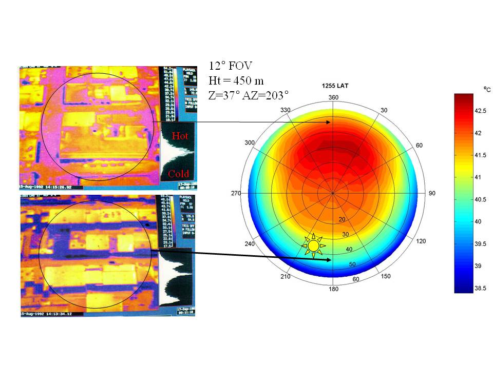
Figure 1. A simple urban surface (A) showing components viewed by nadir (B) and off-nadir (C) remote sensors, and the temperature patterns created by solar loading (D). Voogt and Oke (1998b).

In Figure 2, anisotropy is illustrated using an off-nadir sensor pointed north and southwards across a light industrial district of Vancouver just after solar noon.

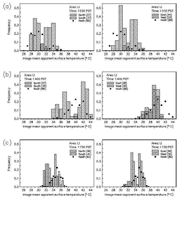
Figure 2. Off-nadir thermal images with temperature frequency distributions towards (top left) the north and (bottom left) the south. Right: polar plot representation of the directional variability of urban surface temperature averaged across a sensor's field of view (represented as the black circles on the thermal images). Thermal images from Voogt and Oke (1998a).

The mean image temperatures differ by over 4°C.

A summary of anisotropy over this type of area is shown by the following histograms of mean image temperature taken at different off-nadir viewing directions (Figure 3).

Figure 3. Histograms of mean image apparent temperature taken during 3 overflights of a light industrial area in Vancouver. From Voogt and Oke (1998a).

Anisotropy of urban surface thermal emissions is strongest during the daytime, but also occurs at night under clear conditions, when the tops of buildings and open areas cool radiatively, while narrow streets and building sides remain warm (Figure 4).

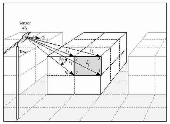
Figure 4. Thermal anisotropy as seen at night over downtown Vancouver from a small off-nadir viewing angle. Darker areas (roof tops) are cooler while building sides and streets near the base of buildings are warmer (lighter shades).

The images above illustrate the problem of defining the urban surface temperature using remote sensors - the temperature observed is complicated by biases related to viewing position, surface geometry and time of day.

A new model (SUM) is available for assessing thermal anisotropy from urban surfaces (Soux et al. 2004).

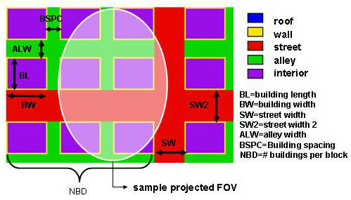
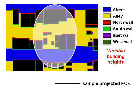
Figure 5. Sensor viewing geometry and view-factor calculation of patches in the SUM (Sun-surface-sensor model) of Soux et al. (2004).

The model can use either a simulated surface geometry, composed of regularly spaced rectangular buildings on a gridded-street system, or can read in actual building footprints and heights from GIS data.

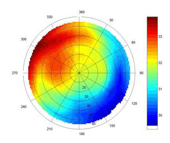
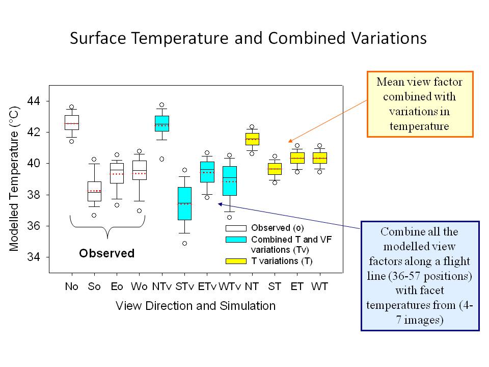
Figure 6. SUM surface geometry options. Top: internal surface geometry with equal building heights. Bottom: building footprints derived from GIS database.

This model can be used in combination with surface temperature information to model the anisotropy from any particular combination of view angle and view direction as shown below. for a mid-morning simulation of the thermal anisotropy over a Light Industrial land use area in Vancouver, BC.

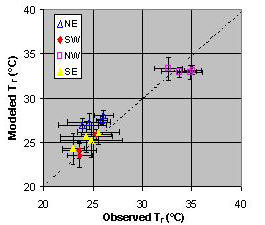
Figure 7. Polar plot of modelled directional radiometric temperature for a 12° FOV thermal sensor at an altitude of 450 m.

A comparison of modelling and observed data for selected view directions over light industrial and downtown areas has been performed. Figure 8 illustrates sample results for downtown Vancouver for a late morning overflight.

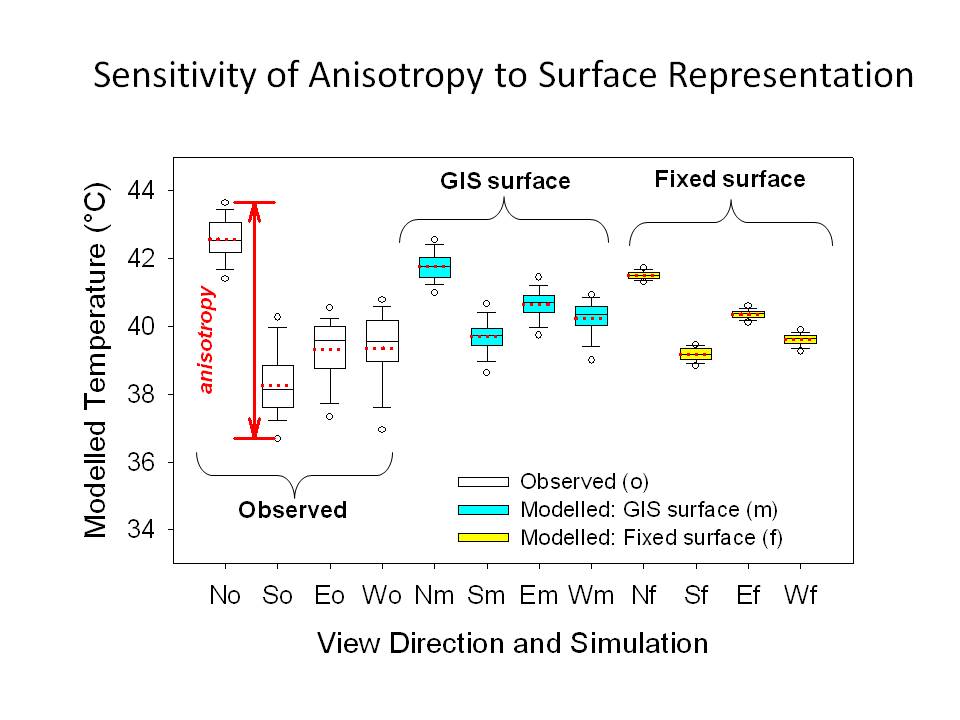
Figure 8. Comparison of modelled and observed directional radiometric temperatures (45° off-nadir view angle, 12°FOV sensor at 525 m) for a downtown area of Vancouver.

Using coupled surface energy balance (e.g. TUF-3D Krayenhoff and Voogt 2007) and the SUM sensor view model, we can perform tests to assess the sensitivity of anisotropy to various forcings.

Figure 9. Sensitivity of modelled directional temperature for North (N), South (S), East (E) and West (W) views over an urban surface to the representation of urban surface structure. The results suggest that anisotropy is due only in part to the surface structure - the use of the actual building footprints relative to a simple equally sized rectangular building improves the the estimation of anisotropy but still falls significantly short of that observed over the study area. After Voogt (2008).

Figure 10. Sensitivity of modelled directional temperature for North (N), South (S), East (E) and West (W) views over an urban surface to temperature variations over the urban surface. The results suggest that small scale variability of urban surface temperature is an important contributor to the overall anisotropy (directional variability) of remotely observed surface temperature (compare to Figure 9). After Voogt (2008).